Nesting Nooks: Exploring Squirrel Habitat & Activity
Every squirrel in Central Park has a very busy schedule. Here, we describe the various activities and tasks squirrels do all over the park, and where those activities occur. Scroll down to learn more about where and when squirrels eat and snacks and get their work done.
#Here we are loading in the data and a shapefile of Central Park!
squirrel_census =
  read_csv("data/clean_squirrel_2018.csv")

central_park_map = st_read(here::here('central_park', 'CentralPark.shp'), quiet = TRUE)
Where do they eat?
Let’s see where all the hungry squirrels are in Central Park!
Each green dot on the map below represents a squirrel that was
spotted eating a snack. Zoom in to explore where squirrels
dine in Central Park!
squirrel_census |>
  filter(eating == TRUE) |> view()
leaflet() |>
  addTiles() |>
  addCircleMarkers(data = squirrel_census,
             lng = ~x,
             lat = ~y,
             label = ~name,
             radius = 1,
             color = "green",
             stroke = TRUE, fillOpacity = 0.75,
             popup = ~paste("Name:", name,
                            "<br> Eating:", eating)) |>
  addProviderTiles(providers$CartoDB.Positron)
There is not a lot of data about what the squirrels were
eating when they were spotted, but here is a list of what
some of the squirrels were spotted snacking on:
- mushrooms
- nuts
- peanuts with shells
- red berries/berries
- osage oranges
- bread
library(rvest)

squirrel_census |>
filter(str_detect(other_activities, "eating")) |>
select(other_activities)
## # A tibble: 20 × 1
##    other_activities
##    <chr>
##  1 eating (ate upside down on a tree — #jealous)
##  2 eating (a mushroom),circles around us,really fat,scratching himself,grooming…
##  3 eating (mushroom)
##  4 eating in tree
##  5 shelling and eating a nut then a dog chased it up a tree & squirrel carried …
##  6 eating loudly <- peanuts w/ shells
##  7 eating (red berries)
##  8 eating (osage orange)
##  9 lying on belly on branch,eating big nut
## 10 eating (nut)
## 11 could this squirrel be eating a white mushroom?
## 12 eating (berries)
## 13 eating (red berries)
## 14 eating upside down on tree trunk
## 15 eating (in a tree)
## 16 eating (a peanut)
## 17 eating bread it found on ground
## 18 eating (nuts)
## 19 eating (in a tree cage thing)
## 20 eating (on branch)
Where do they play?
If the active squirrels aren’t eating, they are surely doing some other activity.
squirrel_census |>
  mutate(
    activity = case_when(
      running == "TRUE" ~ "running",
      chasing == "TRUE" ~ "chasing",
      climbing == "TRUE" ~ "climbing",
      foraging == "TRUE" ~ "foraging",
      .default = "sedentary"
    )
  ) |>
  filter(activity != "sedentary") |>
  ggplot() +
    geom_sf(data = central_park_map, color = "grey") +
  stat_density_2d(
    aes(
      x= x, y= y,
      fill = ..level..
      ),
    geom = "polygon",
    show.legend = TRUE,
    contour = TRUE
  ) +
  scale_fill_viridis_c() +
  scale_alpha_continuous(range = c(0.0, 0.25))+
  theme_void(base_size = 15) +
  theme(legend.position = 'right',
        plot.title = element_text(size = 6))  +
  facet_grid(cols = vars(activity))
## Warning: The dot-dot notation (`..level..`) was deprecated in
## ggplot2 3.4.0.
## ℹ Please use `after_stat(level)` instead.
## This warning is displayed once every 8 hours.
## Call `lifecycle::last_lifecycle_warnings()` to see where
## this warning was generated.
The squirrels can be observed doing every type of squirrel activity
all across the park. There are no bad places to go to watch squirrels
chase each other, climb, forage,
and run! Looking at density plots of where squirrels were
observed doing different activities (above), we see that squirrels seem
to gather en masse to forage around the Central Park Lake,
as shown by the yellow density clustering in the area. Further,
squirrels can commonly be found chasing each other and
running around the southern-most areas of the park.
Up high or down below?
Where should one up high or down low to spot our furry friends?
squirrel_census |>
  ggplot() +
  geom_sf(data = central_park_map, color = "grey") +
  geom_point(
    aes(x = x, y = y, color = location),
    size = 0.5, alpha = 0.75) +
    theme_void(base_size = 15) +
  theme(legend.position = 'bottom') +
  scale_color_viridis_d() +
  guides(color = guide_legend(
    title.position = "top",
    override.aes = list(size = 3))) +
  labs(
       color = "Location")
Our furry friends can most often be seen on the
ground plane, as shown by the yellow points on the map
(left). However, squirrels were also spotted above ground
in the trees all through the park!
Chi-square of location by time of day
Is there a relationship between morning or afternoon sightings
(shifts) and the locations of the squirrels
(ground plane or above ground)?
State Hypotheses
- H0: There is no significant association between
shiftandlocation - H1: There is a significant association between
shiftandlocation
Assumptions
The Chi-Square Test of Independence assumes that
Observations must be independent
Data must be categorical in nature
The expected frequency in each cell in the contingency table should be greater than 5
Data should be collected via random sampling
The overall sample size should be large
We know assumptions 1, 2, 4, 5 and five are met. Let’s double check the cell frequencies by generating a contingency table (below).
#Create contingency table
contingency_table =
  squirrel_census |>
  select(shift, location) |>
  mutate_all(as.factor) |>
  table()
knitr::kable(contingency_table, caption = " A 2x2 table of squirrels seen on or above ground at day or night.")| Above Ground | Ground Plane | |
|---|---|---|
| AM | 417 | 855 |
| PM | 362 | 1190 |
We can see from the contingency table that our cell counts for observed squirrels are well above the required frequency of 5.
Let’s continue on with our chi-square analysis!
# Conduct Test
chi_square_result = chisq.test(contingency_table)
Conclusion
The results of the Chi-Square Test gives us a χ2 value of 30.835 and
a p-value that is smaller than 0.05. At the 5% level of significance,
there is evidence to suggest that the distribution of
locations is not independent of the shift. In
other words, there is a significant association between the time
of day and the location where squirrels are observed.
This may mean that squirrels exhibit different location preferences
or behaviors during the morning (AM) compared to the
afternoon (PM). Squirrels are known to be diurnal animals,
so the results of the chi-square test serves as additional evidence.
Since squirrels have been observed to be active more during dawn and
dusk, this makes a lot of sense.
Regression of location by time of day and activity
We want to see if we can create a logistic regression model to
predict the likelihood of a squirrel being observed on the
ground plane, based on time of squirrel sighting
(shift) and the following behavioral variables:
running, chasing, climbing,
eating and foraging.
# Fitting a Model

set.seed(1)

squirrel_census_df =
  squirrel_census|>
  mutate_all(as.factor)

fit_logistic =
  squirrel_census |>
  glm(location == "Ground Plane" ~ shift + running + chasing + climbing + eating + foraging,
                    data = _,
                    family = binomial())
#Let's tidy up the output.
fit_logistic |>
broom::tidy() |>
mutate(OR = exp(estimate)) |>
select(term, estimate, OR, p.value) |>
knitr::kable(digits = 4)| term | estimate | OR | p.value |
|---|---|---|---|
| (Intercept) | 0.6344 | 1.8858 | 0.0000 |
| shiftPM | 0.4035 | 1.4970 | 0.0003 |
| runningTRUE | 0.7394 | 2.0948 | 0.0000 |
| chasingTRUE | -0.1336 | 0.8749 | 0.4478 |
| climbingTRUE | -2.8895 | 0.0556 | 0.0000 |
| eatingTRUE | 0.3729 | 1.4519 | 0.0058 |
| foragingTRUE | 1.8237 | 6.1945 | 0.0000 |
Based on this output, we see that almost all of our results are
statistically significant at the 5% level. A squirrel spotted on the
ground plane is most likely to be seen
running, climbing, eating, or
foraging. The effect of chasing was not
statistically significant at the 0.05 level. Squirrels spotted on the
ground plane also have a likelihood to be spotted at
night.
Let’s look at some model diagnostics.
squirrel_census |>
  modelr::add_predictions(fit_logistic) |>
  mutate(fitted_prob = boot::inv.logit(pred))
## # A tibble: 2,824 × 38
##        x     y unique_squirrel_id hectare shift date
##    <dbl> <dbl> <chr>              <chr>   <chr> <date>
##  1 -74.0  40.8 13E-AM-1017-05     13E     AM    2018-10-17
##  2 -74.0  40.8 36H-AM-1010-02     36H     AM    2018-10-10
##  3 -74.0  40.8 33F-AM-1008-02     33F     AM    2018-10-08
##  4 -74.0  40.8 21C-PM-1006-01     21C     PM    2018-10-06
##  5 -74.0  40.8 11D-AM-1010-03     11D     AM    2018-10-10
##  6 -74.0  40.8 20B-PM-1013-05     20B     PM    2018-10-13
##  7 -74.0  40.8 22F-PM-1014-06     22F     PM    2018-10-14
##  8 -74.0  40.8 36I-PM-1007-01     36I     PM    2018-10-07
##  9 -74.0  40.8 5C-PM-1010-09      05C     PM    2018-10-10
## 10 -74.0  40.8 7H-AM-1006-05      07H     AM    2018-10-06
## # ℹ 2,814 more rows
## # ℹ 32 more variables: hectare_squirrel_number <dbl>, age <chr>,
## #   primary_fur_color <chr>, highlight_fur_color <chr>,
## #   combination_of_primary_and_highlight_color <chr>, color_notes <chr>,
## #   location <chr>, above_ground_sighter_measurement <chr>,
## #   specific_location <chr>, running <lgl>, chasing <lgl>, climbing <lgl>,
## #   eating <lgl>, foraging <lgl>, other_activities <chr>, kuks <lgl>, …
squirrel_census |>
modelr::add_residuals(fit_logistic) |>
ggplot(aes(x = location, y = resid, fill= location)) +
scale_fill_viridis_d() +
geom_violin() +
theme_bw() +
theme(
legend.position= "bottom"
) +
labs(title = "Distribution of residuals")
squirrel_census |>
  modelr::add_predictions(fit_logistic) |>
  modelr::add_residuals(fit_logistic) |>
  ggplot(aes(x = pred, y = resid)) +
  geom_point(fill= "slateblue2") +
    labs(title = "Residuals vs. Fitted Values",
       x = "Fitted Values",
       y = "Residuals") +
  theme_bw()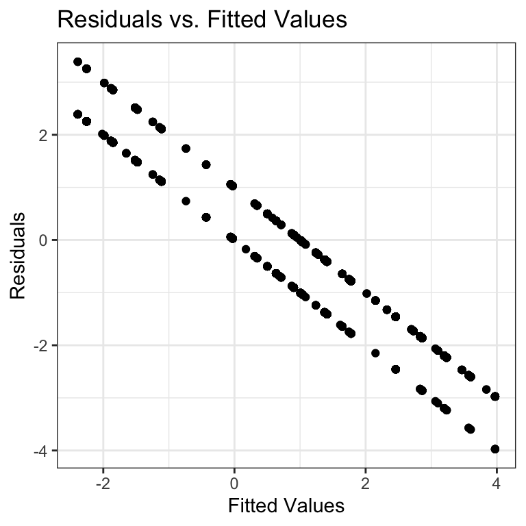
squirrel_census |>
  modelr::add_residuals(fit_logistic) |>
  ggplot(aes(sample = resid)) +
  stat_qq() +
  stat_qq_line() +
  theme_bw()+
  labs(title = "QQ plot of residuals")
From the QQPlot and our residuals plot, this model fit isn’t too awful.